If you are searching examples or an application online on Runge-Kutta methods you have here at our
RungeKutta Calculator
The Runge-Kutta methods are a series of numerical methods for solving differential equations and systems of differential equations.
We will see the Runge-Kutta methods in detail and its main variants in the following sections.
One-step Linear methods
Are numerical methods whose to forward a step, only the previous step information is needed, ie step n+1 only depends on the step n.
Or with more precision, are methods of the form
\(x_{n+1} = x_{n} + F(x_{n}, t_{n}, h) \)
\(x_{0} = x(0) \)
where \(x_{n}\) is a vector of R
n, \(t_{n}\) is the real and independent variable, h the size-step, and F
is a vector function of x
n, t
n, h, ie
\( F: \mathbb{R} ^{n+2}\mapsto \mathbb{R} \)
Note that this problem, is really an equations system.
There are other methods called multi-step, which for to forward a step is required two or more previous steps and there are not linear methods, we will not discuss both kinds of methods here.
Runge-Kutta methods are a specialization of one-step numerical methods . Essentially, what characterizes Runge-Kutta methods is that the error is of the form
$$E_{i}=Ch^{k}$$
Where C is a positive real constant, the number k is called the
order of the method
The Runge-Kutta method number of stages of is the number of times the function is evaluated at each one step i, this concept is important because evaluating the function requires a computational cost (sometimes higher) and so are preferred methods with ao minimum number of stages as possible.
Runge Kutta Methods examples
The Euler Method (Runge-Kutta method with order 1)
$$x_{n+1} = x_{n} + h f(x_{n}, t_{n}) $$
The error is in the form \(e \le = Ch\) and so this method has order 1
Note: The function is one-tme evaluation at each step, so the number of stages is 1.
The middle point rule (Runge-Kutta method with order two)
$$x_{n+1} = x_{n} + h f(x_{n}, + \frac{h}{2}f(x_{n},t_{n}),\, t_{n}+\frac{h}{2}) $$
The error is in the form \(e \le = Ch^{2}\) and so this method has order 2
Note: function are evaluated two times at each step, so stage-number is 2.
Standar fourth-order Runge kutta (Runge-Kutta method with order four)
$$x_{n+1} = x_{n} + \frac{h}{6}(k_{1} + 2k_{2} + 2k_{3} + k_{4})$$
where
\( k_{1} = f(x_{n}, t_{n})\)
\( k_{2} = f(x_{n} + \frac{h}{2} k_{1}, t_{n} + \frac{h}{2})\)
\( k_{3} = f(x_{n} + \frac{h}{2} k_{2}, t_{n} + \frac{h}{2})\)
\( k_{4} = f(x_{n} + h k_{3}, t_{n} + h)\)
Now the error is in the form \(e \le = Ch^{4}\), so the method has order 4
Observation: Stage-number: 4.
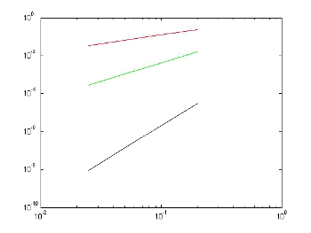
Error grahp size-step h function
|
 |
Error/size-step Graph in logarithmic scale of the tree methods seen here:
- In red, the Euler Method
- In green color the middle point with order 2
- In black, the Runge fourth order Kutta classic
Note the difference in slope, which increases with the order of the method. |
We adopt the following definition as Runge-Kutta Methods:
Runge-Kutta methods definition
A Runge-Kutta method with s-stages and order p is a method in the form
\( x_{n+1} = x_{n} + h \sum_{i=1}^{s}b_{i}k_{i} \)
with
\( k_{i}= f(x_{n} + \sum_{j=1}^{s}a_{ij}k_{j}, t_{n}+hc_{i}) \)
and the error holds the condition
\(Max|x(t_{i})-x_{i}| \le Cht^{p}\)
So, to give a Runge-Kutta Method is necessarily give the s
2 + 2s numbers
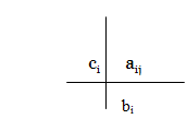
$$b_{i}, c_{i}, a_{ij}$$.
An interesting feature of the Runge-Kutta methods is that it is not needed to calculate derivatives of f to forward. The price to pay for it is to evaluate more times the function f with the consequent
operational cost.
Convergence Theorem for Runge-Kutta methods
Lets F
Lipschitz at x
Then
$$ Max|x(t_{i})-x_{i}| \le \frac{K(e^{Lb} -1)}{L} $$
where L is the
Lipschitz constant of F and k is the truncation local method error.
One method is more efficient if has a reduced number of stages, maintaining order, for example between a 3-stage method with order 3 and one 4-stages of order 3, is much more interesting first one because if we take a step h, the number of calculations to be done will be lower for it.
Butcher Boards
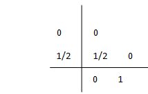
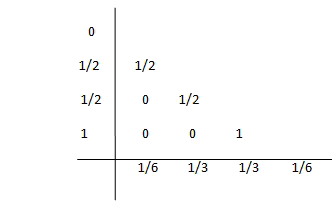
Given a Runge-Kutta, we construct a board as

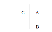
Also it is possible to write as board Butcher

Where A ∈ M
sxs, b ∈ R
s, C ∈ R
s
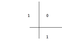
For example, the board Butcher for the Euler method is

For the midpoint rule of order 2

And for the standard Runge-Kutta of order 4

A Runge-Kutta method is said to be consistent if the truncation error tends to zero when Gloval the step size tends to zero.
It can be shown that a necessary and sufficient condition for the consistency of a Runge-Kutta is the sum of bi's equal to 1, ie if it satisfies
$$1=\sum_{i=1}^{s}b_{i}$$
In addition, the method is of order 2 if it satisfies that
$$ 1= 2\sum_{j=1}\sum_{i=1}^{s}a_{i}b_{j} $$
Similar conditions can be given for methods with orderers 3, 4, ...
Explicit Runge-KuttaMethods
In a Runge-Kutta explicit, given in the ki
the definition does not appear as a function of them
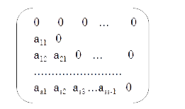
themselves are clear The matrix a in the Butcher board is "almost inferior triangular" because it is inferior triangular and the diagonal elements are zero too.

Theorem
A Runge-Kutta explicit method with s-stages may nor have order higher than s.
It is known that there are not Runge-Kutta explicit methods with s stages with order s for s greater than or equal to 5
It is also known that there aren't Runge-Kutta explicit s-stage order s-1, for s greater than or equal that 7.
More generally we have the following table

That step size is necessary? The answer to this question is that
depends on the specific problem and the desired degree of accuracy.
One thing to consider is that Runge-Kutta methods lose some precision when the derivative of the function analysis is very large or frequently changing sign, such cases requires a very small step size to obtain an acceptable degree of accuracy
At next section we will see the
Fehlberg Pairs embebbed , are methods in which the step size
will vary automatically depending on (among other things) of changes in the derivative of the function
If you want to see now an example of how these methods works, access to
RungeKutta Calculator where you will see the default problem
$$ \left\{\begin{matrix} y'=f(x,y) & \\ y(x_{0})=y_{0} \end{matrix}\right. $$
Whose exact solution is obviously \(y=e^{x}\).


